
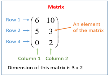
Matrices in mathematics are rectangular arrays of numbers, expressions, or symbols organized in columns and rows. For example, the matrix below is 3 × 2 pronounced as “three by two”, because there are three rows and two columns:
The number of columns in the first matrix (A) must equal the number of rows in the second matrix (B) when multiplying matrices. The result which is the product of the two matrices is known as the matrix product which is in a dimension of the number of rows of the first and the number of columns of the second matrix that is a 2×3 matrix can multiply a 3×2 matrix to give a result of 2×2 matrix and the product of matrices A and B is given to be AB.
Multiplying large sizes of a matrix has been a great challenge for researchers but yet endless research continues to approach a faster method of multiplication. It’s possible and easier to multiply two matrices of compatible sizes to produce a third matrix without error than multiplying matrices with large sizes. When multiplying a pair of two-by-two matrices, the result produced will be in a two-by-two matrix structure with four entries. In general, a pair n-by-n matrices multiplied will produce another n-by-n matrix with n² entries, where n is 2 it has 2² entries giving 4 entries in total.
The ideal pace of conducting one of the most fundamental operations in math, matrix multiplication, is often referred to as “exponent two”. Exponent two means multiplying pairs of matrices in n² steps where n² steps are the number of steps it takes to write down the result of the multiplication. Mathematicians have been working hard to reach the goal of using exponent two to achieve faster multiplication of matrices. The opinion on “exponent two” reduce to a feeling of how the world ought to be for computer scientists and mathematicians.
The closest approach so far is reported in a paper published in October 12, 2020, which describes the fastest method for multiplying two matrices together ever devised. Josh Alman, a Harvard University postdoctoral scholar, and Virginia Vassilevska Williams, of the Massachusetts Institute of Technology, came up with a solution that reduces the exponent of the previous best mark by around one-hundredth. It is an indication of the field’s recent strenuous progress.
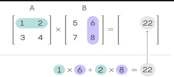
For a better understanding of the progress and improvement given an example of the multiplication of two 2×2 matrices A and B. To compute each entry of their product, you use the corresponding row of A and the corresponding column of B. To get the top-right entry, multiply the first number in the first row of A by the first number in the second column of B, then multiply the second number in the first row of A by the second number in the second column of B, and add the two products together.
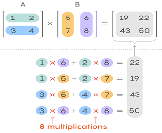
Repeat the process with the corresponding rows and columns to compute the remaining entries in the product matrix. Taking the “inner product” of a row and a column is what this operation is called. The education method for multiplying a pair of 2×2 matrices involves eight multiplication and four additions.
The larger matrices grow the more the numbers of multiplication and addition are required to find their product but the number of multiplication increases faster than the number of addition. As said earlier, the multiplication of a pair of 2×2 matrices will take eight multiplication while that of 4×4 matrices will take 64 multiplication to find its product. The number of additions needed to add such sets of matrices, on the other hand, is much closer. The number of additions is usually equal to the number of entries in the matrix, which is four for two-by-two matrices and sixteen for four-by-four matrices. This distinction between addition and multiplication explains why matrix multiplication speed is measured solely in terms of the number of multiplications needed.
For decades, people assumed that n³ was actually the quickest way to multiply matrices. Volker Strassen is said to have set out in 1969 to prove that multiplying two-by-two matrices with less than eight multiplications was impossible. He couldn’t seem to find the evidence, and after a while, he realized why which is because there is a way to do it with only seven multiplication. Strassen came up with a theory that replaces one multiplication with 14 addition providing just seven multiplication needed with 18 addition to getting the matrix result. While it does not seem to make a significant difference, it is better because multiplication is more important than addition. Strassen discovered an opening when multiplying larger matrices by discovering a way to save a single multiplication for small two-by-two matrices.
For instance, suppose you want to multiply two eight-by-eight matrices. One process is breaking each large matrix into four four-by-four matrices, each with four entries. Since matrices can have entries that are also themselves, the original matrices can be thought of as a pair of two-by-two matrices, each of whose four entries is a four-by-four matrix. These four-by-four matrices can be broken down into four two-by-two matrices with some manipulation. The advantage of repeatedly splitting larger matrices into smaller matrices is that Strassen’s algorithm can be applied to the smaller matrices over and over again, reaping the benefits of his method at each step. Overall, Strassen’s algorithm reduced the number of multiplicative steps in matrix multiplication from n^3 to n^2.81.
In the late 1970s, the next significant advancement occurred with a radically different approach to the issue. It entails converting matrix multiplication into a separate linear algebra computational problem involving tensors. Tensors are three-dimensional arrays of numbers made up of several different components, each of which looks like a small matrix multiplication problem. In certain ways, matrix multiplication and this tensor problem are the same things, but researchers already had faster methods for solving the tensor problem leaving them with the task of calculating the exchange rate between the Matrix multiplication and Tensor. The major question is how large are the matrices you can multiply for the same computational cost as solving the tensor problem?.
This approach was used in 1981 by Arnold Schönhage to prove that it’s possible to perform matrix multiplication in n2.522 steps which were later named the “laser method”. Researchers have been working on the ” laser method” over the last few years to improve matrix multiplication and discovered efficient ways to translate between matrix multiplication problems. Alman and Vassilevska Williams demonstrate that it is possible to “buy” more matrix multiplication than previously realized for solving a tensor problem of a given size in their new proof by reducing friction between the two problems.
Despite all the maneuvering, it’s clear that this method is yielding diminishing returns. In particular, Alman and Vassilevska Williams’ progress may have nearly reached the theoretical limit of the laser method, but not meeting the ultimate theoretical target. The theoretical speed limit for matrix multiplication is improved to n^2.3728596 in this paper. It also helps Vassilevska Williams to reclaim the matrix multiplication title she previously held in 2012 (n^2.372873) before losing to François Le Gall in 2014. (n^2.3728639).
References
https://en.m.wikipedia.org/wiki/Matrix_(mathematics)
https://www.quantamagazine.org/mathematicians-inch-closer-to-matrix-multiplication-goal-20210323/


